To reach centimeter-level — or even better — accuracy of positioning typically requires use of precise dual-frequency carrier phase observations. Furthermore, these observations are usually processed using a differential GNSS (DGNSS) algorithm, such as real time kinematic (RTK) or post-processing (PP). Regardless of the specific differential algorithm, however, implicit in the process is an assumption that the quality of the reference station data is consistent with the desired level of positioning accuracy. As a quick review, a typical DGNSS setup consists of a single reference station from which the raw data (or corrections) are sent to the rover receiver (i.e., the user). The user then forms the carrier phase differences (or corrects their raw data) and performs the data processing using the differential corrections.
In contrast, GNSS network architectures often make use of multiple reference stations. This approach allows a more precise modeling of distance-dependent systematic errors principally caused by ionospheric and tropospheric refractions, and satellite orbit errors. More specifically, a GNSS network decreases the dependence of the error budget on the distance of nearest antenna.
Types of Real-Time Network Correction Services available within SLCORSnet
SLCORSnet comprises of state-of-the-art software solution from GEO++ GmbH that is independent of all hardware manufacturers. The system primarily operates on GEO++ GNSMART GNSS Network software which is currently the most advanced network software available commercially and GEO++ GNSMART was also the first solution in the market to introduce and provide VRS corrections to the general public in 1995. Hence today, SLCORSnet is capable of providing all available real-time correction techniques as explained in detail below. The below given information should help you better understand the different real-time correction methods and their main differences.
VRS
Virtual Reference Station
The Virtual Reference Station (VRS) concept can help to satisfy this requirement using a network of reference stations.
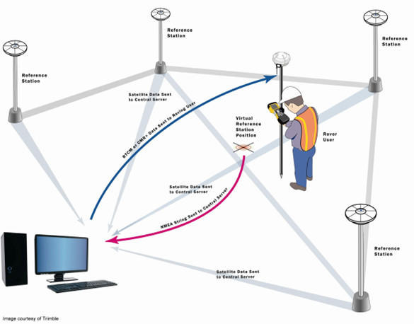
The general concept of network-based processing is shown in Figure 1(above). The network of receivers is linked to a computation center, and each station contributes its raw data to help create network-wide models of the distance-dependent errors. The computation of errors based on the full network’s carrier phase measurements involves, first of all, the resolution of carrier phase ambiguities and requires knowledge of the reference station positions. (The latter is usually determined as part of the network setup.)
At the same time the rover calculates its approximate position and transmits this information to the computation server, for example, via GSM or GPRS using a standard National Marine Electronics Association (NMEA) format. The computation center generates in real time avirtual reference station at or near the initial rover position. This is done by geometrically translating the pseudorange and carrier phase data from the closest reference station to the virtual location and then adding the interpolated errors from the network error models.
This generated VRS data is then sent to the user through a wireless connection, often using the Networked Transport of RTCM via Internet Protocol (NTRIP). Finally, just as if the VRS data had come from aphysical reference station, the rover receiver uses standard single-baseline algorithms to determine the coordinates of the user’s receiver, in near-real-time kinematic or post-processed modes.
PRS
Pseudo Reference Station
PRS refers to Pseudo Reference Station where the virtual reference station is always placed at a predefined fixed distance from the rover position.
The correction methodology works the same as for VRS as explained above.
This correction is specifically developed to work well with the older models of rovers which were not specifically designed to work within GNSS networks and more specifically VRS corrections. This method allows the rovers to consider the overall error budget in its RTK computation algorithms.
FKP
Flächen Korrektur Parameter
With FKP methodology, a model of the distance dependent errors (“Flächen-Korrektur-Parameter” FKP) is transmitted to the rover. The interpretation of the FKPs and the individualization of the corrections are done at the rover, i.e. the rover can for itself compute the individualized corrections in the same way as VRS/PRS or alternatively use its own algorithms, which might be better adjusted to the RTK algorithms of the rovers. Thus the FKP method provides to the rover more information than VRS method, so that the rover in principal can get more from the received data.
FKPs describe the (horizontal) gradients of the corrections. The correction of a (real) reference station is used in combination with the FKPs to compute the individualized corrections for the rover position.
In the simplest case the FKPs describe a linear dependency of the corrections from the position (linear FKP). The FKPs then define an “inclined plane” for the corrections, centered at the (real) reference station. Per satellite and per frequency two parameters (inclination in North-South and in West-East) are required. FKP models of higher order are possible. Note that the validity of linear FKP is limited to about 100km radius, due to the fact that the physical error sources would lead to noticeable non-linear effects over longer distances.
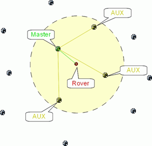
MAC
Master Auxiliary Concept
MAC (Master-Auxiliary-Concept) uses phase correction difference of one master station with multiple auxiliary stations. Normally the rover sends its position to the central office which determines the next available network station as master station. Then coordinate differences between master and auxiliary stations and geometric/ionospheric correction differences are send out back to the rover. The computation and adjustment of final correction data (individualization) is done on the rover which requires therefore additional software (algorithm) and processing (CPU) resources.
The validity area of MAC is the area covered by the master and all auxiliary stations.
MAC is rather equivalent to FKP. Both use the output for the master station, which is unchanged compared to a single (stand-alone) reference station, and add information about spatial variations of the corrections. FKP sends these spatial variations as ppm values in North and East direction. MAC sends the spatial variations for discrete points (i.e. auxiliary stations).
One general distinction between MAC and VRS/PRS is the location where correction data is individualized. The VRS/PRS individualization for the user position is computed in the central office for a location near to the real rover position and is provided by the correction data provider. For MAC the individualization must be done on the rover itself within an adjustment or interpolation, which needs especially additional resources and algorithms in the rover. An adjustment method is not defined by RTCM and the realization on the rover can be manufacturer dependent. For VRS/PRS the computation is always the same and based on formulas which are used for all rovers.
MAC also needs more bandwidth than RTCM3 VRS/PRS due to the transmission of multiple station information (additional message types 1014, 1017, 1039). But on the other hand MAC can provide a theoretical higher redundancy.
The achievable accuracy for MAC and VRS should be generally the same. VRS/PRS is possible with RTCM2 and RTCM3. MAC is only possible with RTCM3, where MAC for GPS is RTCM3-standardized since 2006, MAC for GLONASS since 2011. At the moment, VRS is supported by nearly all rovers, whereas older rovers often don’t support MAC, or support MAC only for GPS.
Sri Lanka Continuously Operating Reference Station Network